Sigmoid, Softmax and Logistic Regression: From Scores to Probabilities

Almost every classifier ends the same way: it produces some raw numbers and then converts them into probabilities. Two functions do that conversion, the sigmoid and the softmax, and the model that uses them in its simplest form is logistic regression. They are usually taught separately, but they are really one idea. This article connects them, shows the small amount of maths that matters, and explains where each one appears inside modern deep learning and language models.

If you are new to logistic regression, our earlier article What Is Logistic Regression? introduces it with text and image examples. Here we go one level deeper into how it produces and learns probabilities.

The setting: scores in, probabilities out

A logistic regression model first computes a score (often called a logit) as a weighted sum of the features: z = w1·x1 + w2·x2 + ... + b. That score can be any number, from very negative to very positive. A score is not a probability, so we need a function that maps it into the range 0 to 1. For two possible answers, that function is the sigmoid. For many possible answers, it is the softmax.

The sigmoid: one score, two outcomes

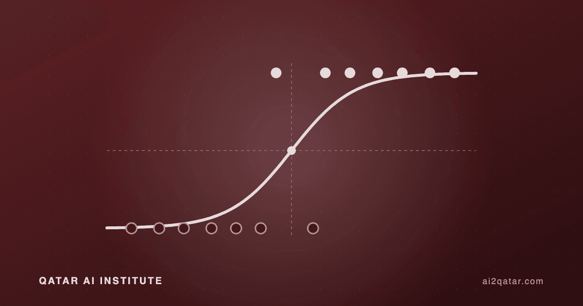
The sigmoid is σ(z) = 1 / (1 + e−z). Its useful properties:

• Range: always strictly between 0 and 1, so it can be read as a probability.
• Midpoint: σ(0) = 0.5. A score of zero means "no idea".
• Symmetry: σ(−z) = 1 − σ(z). The probability of "no" is simply what is left over.
• Gradient: its slope is σ(z)·(1 − σ(z)), at most 0.25 and close to zero when the model is very sure. We will see why that matters below.

The sigmoid also gives the score a meaning. Rearranging it gives z = ln( p / (1 − p) ), the log-odds of the answer. So each weight is the change in log-odds for a one-unit change in its feature, and ew is the factor by which the odds are multiplied. That is why logistic regression is easy to interpret: a weight of 0.7 on a feature means the odds go up by a factor of about 2 (e0.7 ≈ 2.01) when that feature increases by one.

The softmax: many scores, one distribution

With more than two classes, the model computes one score per class, and the softmax turns the list of scores into a list of probabilities: softmax(z)i = ezi / Σj ezj. It works in three steps:

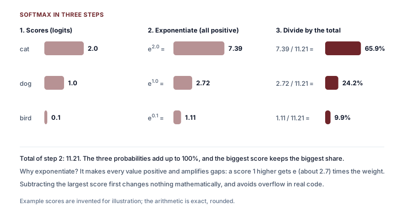
• Exponentiate each score, which makes everything positive and widens the gaps (a score one point higher gets about 2.7 times the weight).
• Add them up to get a total.
• Divide each value by the total, so the results add up to exactly 1.

Two more properties are worth knowing. Softmax never changes the order: the largest score always gets the largest probability. And adding the same constant to every score changes nothing, which is why real code subtracts the largest score first to avoid numerical overflow.

They are the same thing

Take a softmax with two classes and fix the second score at 0. Then the probability of the first class is ez / (ez + e0) = ez / (ez + 1). Divide top and bottom by ez and you get 1 / (1 + e−z), which is the sigmoid.

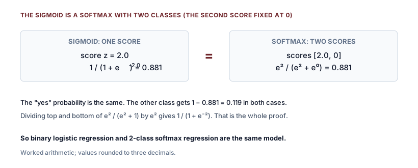
So binary logistic regression (sigmoid) and multi-class "softmax regression", also called multinomial logistic regression, are one model family. The only difference is how many scores you compute.

Which one to use: multi-class or multi-label?

The choice is about the question you are asking, not about the number of outputs:

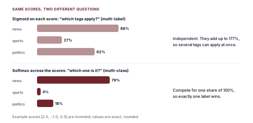
• Softmax when the classes are mutually exclusive: a handwritten digit is exactly one of 0 to 9, a review has one sentiment. The classes compete for a fixed 100%.
• A sigmoid per class when labels can co-occur: an article can be tagged "news" and "politics" at once, a chest X-ray can show several findings. Each label is its own yes/no question, and the probabilities do not need to add up to 1.

How the model learns: cross-entropy

Training needs a number that says how wrong the predicted probabilities are. For both the sigmoid and the softmax, the standard choice is the cross-entropy loss: take the probability the model gave to the correct answer and compute −ln(p). If the model gave the right class 100%, the loss is 0. If it gave it 1%, the loss is about 4.6. Confident mistakes are punished heavily.

Using the cat, dog and bird example, suppose the true answer is "cat". The model gave it 65.9%, so the loss is −ln(0.659) ≈ 0.417. And the gradient of the loss with respect to each score has a strikingly simple form: predicted probability minus the true label. Here that is [0.659 − 1, 0.242 − 0, 0.099 − 0] = [−0.341, +0.242, +0.099]. In plain terms, the update raises the cat score and lowers the other two, in proportion to how wrong each one was. The same p − y rule holds for the sigmoid with its two outcomes. This simplicity is a big reason these pairings (sigmoid or softmax plus cross-entropy) are used everywhere, and why the gradient does not shrink when the model is confidently wrong, as it would with a squared-error loss.

Temperature: reshaping the distribution

You can divide the scores by a number T, the temperature, before applying the softmax. It does not change the ranking, but it changes how sharp the distribution is:

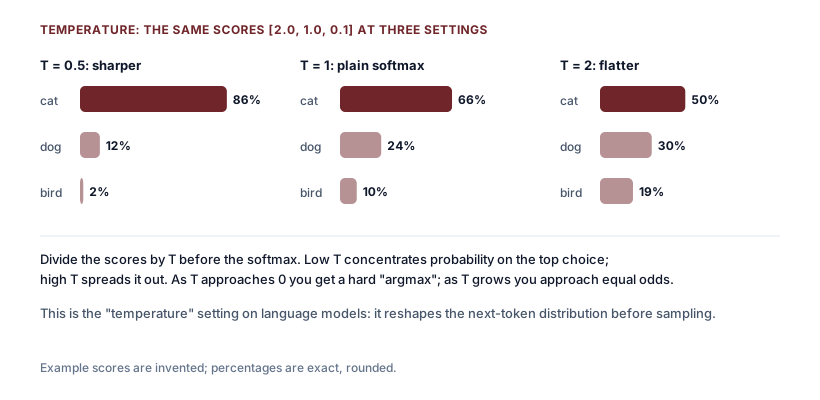
This is exactly the "temperature" setting you see in language-model tools. A low temperature makes the model pick its top choice almost every time; a high temperature spreads the probability out and makes the output more varied.

Where you meet them in deep learning

A recent example: Liquid AI's d1 "decision models" return probabilities instead of text. See Liquid AI d1: AI Models That Decide Instead of Writing.

• The last layer of a classifier. An image network that outputs 1,000 class scores ends in a softmax. A binary classifier ends in a sigmoid. Everything before that layer learns features; the last layer is logistic regression on those features.
• Language models. At every step, a language model computes a score for each token in its vocabulary and applies a softmax to get the next-token distribution, from which a token is sampled (see What Is a Transformer?). A related mixture-of-experts router also uses a softmax-style choice to decide which experts to use.
• Attention. Inside a transformer, the attention scores between words are turned into weights that add up to 1 with a softmax, so each word spreads one unit of attention over the others.
• Masked-word prediction. Models such as BERT and the diffusion models in our ALoDLM explainer use a softmax over the vocabulary at each masked position.

A small implementation

import numpy as np

def sigmoid(z):
    return 1 / (1 + np.exp(-z))

def softmax(z):
    z = z - np.max(z)          # subtract the max: same result, no overflow
    e = np.exp(z)
    return e / e.sum()

scores = np.array([2.0, 1.0, 0.1])
p = softmax(scores)            # [0.659, 0.242, 0.099]

y = np.array([1, 0, 0])        # the true class is "cat"
loss = -np.log(p[0])           # cross-entropy: 0.417
grad = p - y                   # gradient wrt the scores: [-0.341, 0.242, 0.099]

# The sigmoid is a two-class softmax:
print(sigmoid(2.0), softmax(np.array([2.0, 0.0]))[0])   # both 0.881

Common pitfalls

• Overconfidence. A softmax output is not automatically a calibrated probability. Deep networks are often more confident than they are accurate, so "95%" may not mean right 95% of the time. Calibration methods exist to fix this.
• No "none of the above". Softmax must give all its probability to some class, even for an input that fits none of them. Out-of-scope inputs need a separate check, such as a confidence threshold or an extra "other" class.
• Saturation. Because the sigmoid's slope is at most 0.25 and nearly zero at the extremes, stacking many sigmoid layers makes gradients vanish. This is why hidden layers in modern networks use functions like ReLU, and the sigmoid is kept mainly for the output.
• Numerical stability. Computing ez directly for large scores overflows. Subtract the maximum first, and in training use the library's combined "softmax cross-entropy" function, which handles this for you.

Key takeaways

• Logistic regression computes a score and turns it into a probability.
• The sigmoid handles two outcomes; the softmax handles many, and the sigmoid is a two-class softmax.
• Use softmax for "which one?" and sigmoids for "which of these apply?".
• Cross-entropy with either gives the clean gradient p − y.
• Temperature divides the scores before the softmax and controls how sharp the distribution is.

To go from these ideas to a working model, see our 7 machine learning algorithms every beginner should know, and build logistic and softmax regression from scratch in our Machine Learning Fundamentals course.